Intro
A computer tomography scan is a medical imaging system that shoots x-rays through a body from many different angles.
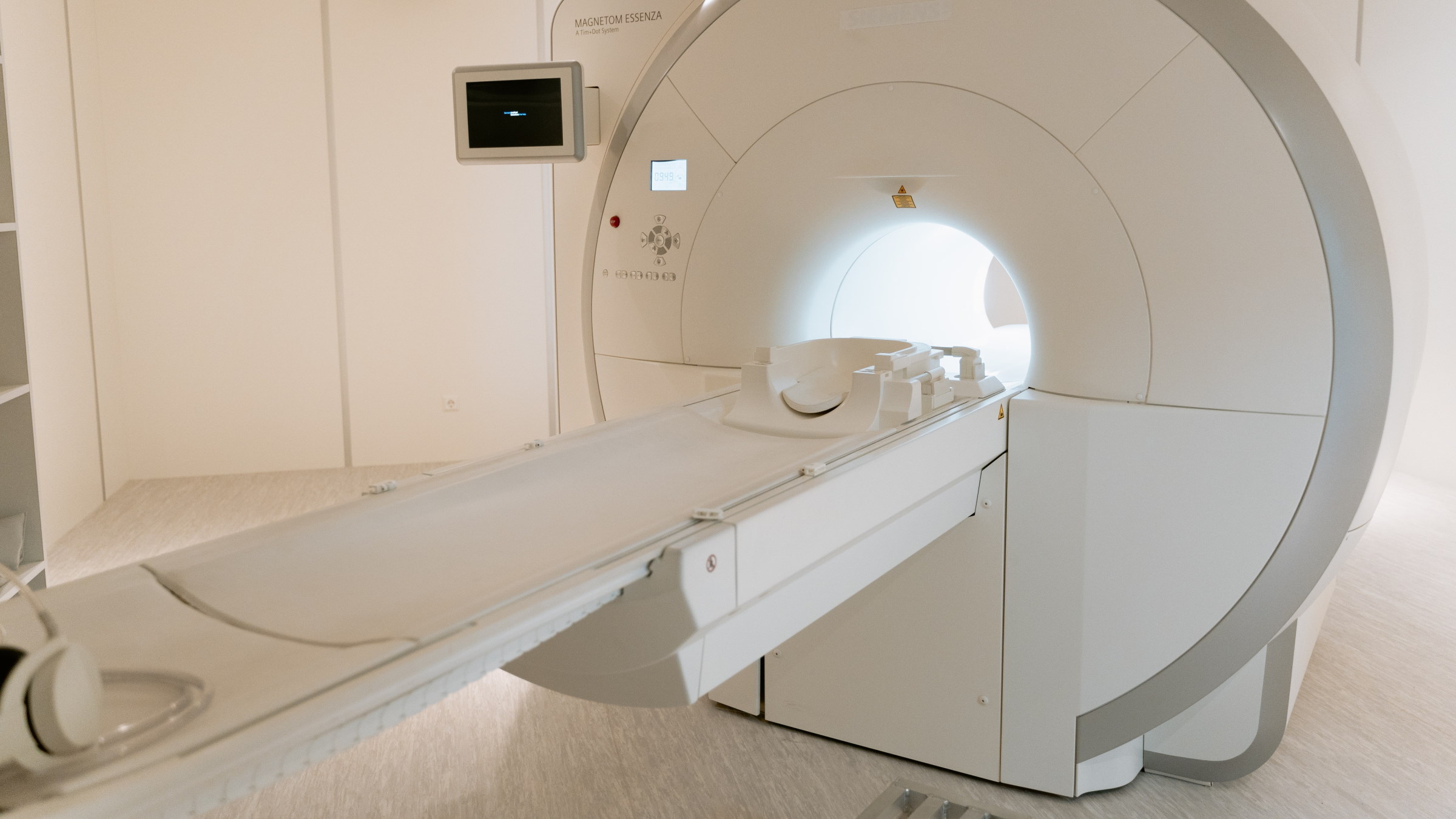
From these x-rays, we can construct an image of how the body looks on the inside. But have you ever wondered how the image is actually constructed?
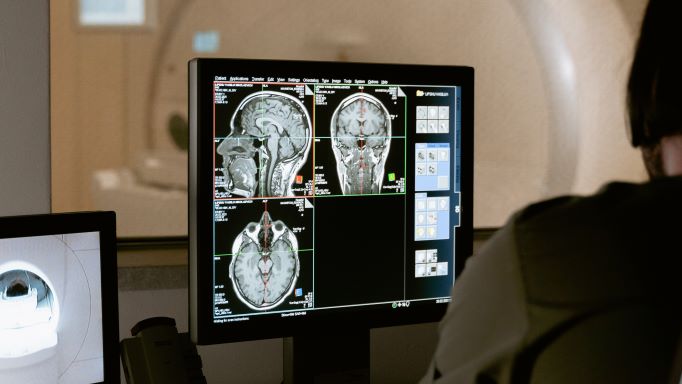
The answer is of course with mathematics, specifically with the so called Radon transform. The Radon transform is a type of integral transform, which is a general linear transformation.
Concept
Look at the following two functions:
which both take real numbers as inputs, and produces, as output, new real numbers along straight lines with slopes of , intersecting the y-axis at and respectively.
However, only one of the functions is in fact linear.
For a function to qualify as linear, it must satisfy two properties:
Additivity:
Homogeneity:
where is any scalar.
This holds true for , but not for , as we will see later.
General linear transformations must satisfy the same two properties, only that instead of real numbers, they are functions from one vector space to another.
Math
Let and with
Now is both additive and homogeneous:
Further, we can show that is neither additive or homogeneous with a simple example. Let , then:
Consequently, is linear whereas is not.
We have to go through he same process to determine whether a transformation , where and are vector spaces, is a linear transformation or not.
General linear transformations
Introduction
Having relaxed the concept of vector space, we are ready for a similar generalization of linear transformations. This lecture note is usually easier for students to digest, as the mental leap has already been taken for the general vector spaces. Therefore, we dive directly through the following definition of linear transformations:
The definition
Let
be a function from a vector space to a vector space , then is called a linear transformation from to , if the following two properties hold for all vectors and for all scalars :
, \quad (homogeneity)
, \quad (additivity)
For the special case when the two vector spaces are equal, meaning , is called a linear operator on vector space .
Consequently, we have the three following results for a linear transformation :
Before we move on, let's look at the definitions for kernel and image (or range) respectively:
Let be a linear transformation. We then have two sets of vectors, called the kernel and image of respectively, and we define them as:
The kernel is the set of vectors in that maps into , and we denote it by .
The image, or range, is the set of vectors in that are images of at least one vector in , and we denote it by .
Three theorems
Three useful theorems are hereby listed. They can be used for solving problems or proving other theorems.
If is a linear transformation, then maps subspaces of into subspaces of .
If is a linear transformation, then is a subspace of and is a subspace of .
If is a linear transformation, then the following are equivalent:
is one-to-one
We now visit five examples of linear transformations, namely zero transformation, identity transformation, evaluation transformation, differentiation transformation and integral transformation.
Zero transformation
Let and both be vector spaces and let us consider the transformation:
where
which means that each vector in is transformed to the zero vector . This transformation is in fact linear, since we have for every scalar :
Identity transformation
Let and both be vector spaces and let us consider the transformation:
where
which means that each vector in is transformed to itself. This transformation is in fact linear, since we have for every scalar :
Evaluation transformation
Let be a subspace of the vector space and consider the following sequence of distinct real numbers:
We have the following mapping that associates with its -tuple of function values at the aforementioned sequence:
where
We call this the evaluation transformation on at
For example, if we have that
and if we let
we then get:
The evaluation transform is linear, since we have for every scalar :
Differentiation transformation
Let be the vector space of real-valued functions with continuous first derivatives on . Further more, let be the vector space of continuous real-valued functions on . Let us now consider the following linear transformation,
which is the transformation that maps a function to it's first derivative.
This transformation is in fact linear, since we have for every scalar the following differentiation rules from calculus (not proven here):
We can generalize this transformation by introducing , the k:th derivative of , and the vector space . Then we have that
where is the same vector space as before and
Integral transformation
Let
be the vector space of continuous functions on . Further more, let
be the vector space of functions with continuous first derivatives on . Let us now consider the following linear transformation,
which is the transformation that maps a function to the integral:
This transformation is in fact linear, since we have for every scalar the following integration rules from calculus (not proven here):
Isomorphism
Introduction
Isomorphism is a recurring concept within mathematics, and depending on area in mathematics it is known by specialized names, such as isometry for metric spaces, homeomorphism for topological spaces, diffeomorphism for differentiable manifolds and automorphism for permutations of a set. It is not necessary to understand all of these concepts for a course in linear algebra, but students who are inspired to study higher mathematics will become familiar with one or more of these. Mathematics is a truly beautiful, like a science art.
Definition
So, let's get to the point and define isomorphism:
Let's say we have a linear transformation , and the two vector spaces and , such that
that is one-to-one (each vector maps to a unique vector in ) and onto (all vectors that pairs with at least one vector in under ). Then we call an isomorphism, and we say that the vector space is isomorphic to the vector space .
Most of our theorems have been focused on the real vector space , which may seem limited for the true abstract thinker. In fact, all of these theorems are still valid thanks to a beautiful theorem with a simple proof. The theorem states that all n-dimensional vector spaces are isomorphic to . Before we state the theorem and show the proof, we will dip our toes in this water by building some kind of intuition for the stated problem. Let us compare the polynomial space to the real vector space . We then have that each polynomial can be expressed uniquely in the form:
and can therefor be uniquely represented by its n-tuple of coefficients:
Thus, we have a trivial transformation such that:
Since each possible combination of coefficients
can trivially be related to each vector in we have that is a one-to-one and onto mapping from to . We also have that is linear, since we have for every polynomial and :
and for each scalar that:
So we have shown to be a linear transformation from to , and justified why it is one-to-one and onto. Hence, is an isomorphism, and after this toe-dip we are now ready for the following beautiful theorem, with accompanying simple proof:
Every real -dimensional vector space is isomorphic to
Let be a real -dimensional vector space. We prove to be isomorphic to by finding a linear transformation
that is one-to-one and onto. We start by defining a basis for :
This means we have for every vector a unique linear combination such as:
where are the coordinates of with respect to the basis . We now define the transformation :
so that we have that:
Of course, this transformation is not randomly selected. We have an intuition for it to meet the requirements of an isomorphism. To show this, we need to prove is linear, one-to-one and onto. We show these three properties one at a time. We start by showing linearity:
Linearity (1/3)
Let and be vectors in such that
and let be a scalar. We show the two properties of linearity:
One-to-one (2/3)
Now we show to be one-to-one, and we do that by showing that if and are distinct vectors, then so are their images under . Since:
which shows that and have distinct images under .
Onto (3/3)
Finally, we show that is onto by assuming belonging to with components:
which must be an image under of the vector such that:
This concludes the proof.